If you’ve ever scrolled through a huge Excel spreadsheet and lost track of crucial data, you know how frustrating it can be. Freezing rows in Excel is an incredibly useful trick to solve this problem. But what if the row you need to freeze isn’t the top one? No worries!
In this guide, we’ll walk you through how to freeze a row in Excel that is not the top row, ensuring that the important information you need stays visible as you navigate through your data.
By the end of this article, you’ll master how to keep any specific row locked in place, making your Excel experience smoother and more efficient.
What Does It Mean to Freeze a Row in Excel?
Before we dive into the specific steps, let’s quickly cover what freezing a row in Excel actually does. Freezing a row locks it in place, so even when you scroll down your spreadsheet, the frozen row remains visible. This is particularly useful when working with large datasets where headers or key rows contain vital context.
For instance, freezing rows helps you:
- Maintain context when you’re scrolling through endless rows of data.
- Improve readability by keeping labels or important information in view.
- Enable quick comparison between different rows and key data points.
Step-by-Step Guide: How To Freeze A Row In Excel That Is Not the Top Row
Freezing rows that are not at the top is slightly different from freezing the first row, but it’s just as simple once you get the hang of it. Here’s how to do it:
1. Select the Row Directly Below the One You Want to Freeze
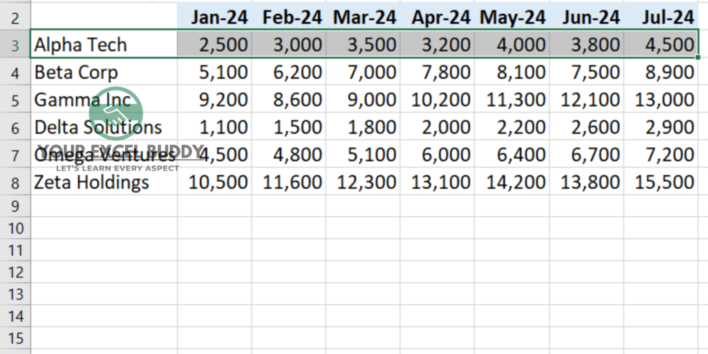
If you want to freeze, let’s say, row 5, you need to select row 6. This tells Excel to freeze all rows above your selected row.
Example: Want to freeze row 5? Click on row 6.
2. Go to the View Tab on the Excel Ribbon
Navigate to the Excel ribbon at the top of your screen, and click on the View tab. This is where you’ll find the option to freeze panes.
3. Open the Freeze Panes Dropdown
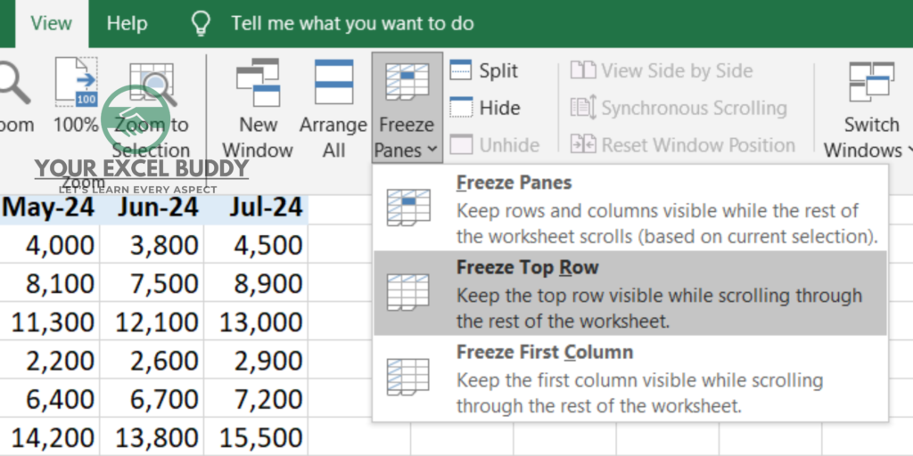
In the View tab, locate the Freeze Panes button. Click it, and a dropdown menu will appear with different options.
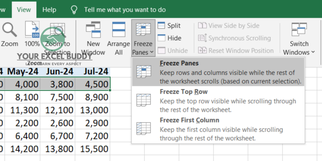
4. Choose the “Freeze Panes” Option
From the dropdown, select Freeze Panes (not the “Freeze Top Row” option). This will lock all rows above the one you selected.

Tip: This method works for any row that isn’t at the top of the spreadsheet. If you selected row 6, then rows 1 through 5 will stay locked in view as you scroll through the rest of the worksheet.
Best 119+ Excel Shortcuts Cheat Sheet For Excel Users
Alternative: Freezing Multiple Rows That Are Not the Top Row
Maybe you want to freeze more than just one row at the top or a random row in the middle. Here’s how you can freeze multiple rows in Excel:
1. Select the Row Below the Last Row You Want to Freeze
Let’s say you want to freeze rows 3, 4, and 5. You need to select row 6. Selecting this row will freeze everything above it.

2. Go to the View Tab
Again, head over to the View tab at the top of your screen.
3. Click on Freeze Panes
From the Freeze Panes dropdown, choose Freeze Panes to lock the selected rows in place.

This will freeze rows 3, 4, and 5, and they will remain visible even as you scroll down the sheet.
How To Freeze A Row In Excel Using a Keyboard Shortcut
Prefer using keyboard shortcuts? Excel’s got you covered! You can freeze panes with just a few key presses.
1. Select the Row Below the One You Want to Freeze
Just like before, click on the row beneath the one you want to lock.
2. Use the Keyboard Shortcut
Press the following keys in sequence:
Alt + W + F + R
This shortcut will immediately freeze the selected rows, locking all rows above the one you clicked on.
Unfreezing Panes in Excel: A Quick How-To
If you no longer need the rows frozen and want to unfreeze your spreadsheet, it’s easy to undo the action.
1. Go to the View Tab
Click on the View tab at the top of your Excel screen.
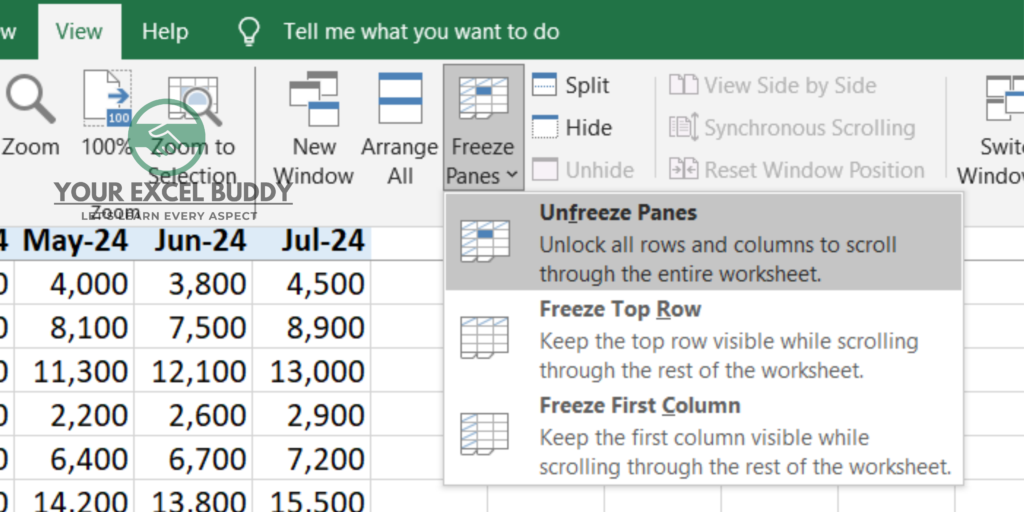
2. Click on Freeze Panes
From the Freeze Panes button dropdown, select Unfreeze Panes. This will remove any frozen rows and return your spreadsheet to its original state.

Top 20 Importance of Excel in Finance: Essential Skills for Every Finance Professional
To Sum Up: Master Your Excel Workflow with Frozen Rows
Now that you know how to freeze a row in Excel that is not the top row, navigating through large spreadsheets should be much easier. By keeping important rows in view, you can focus on the data that matters without losing track of headers or key information.
Whether you’re using the menu or keyboard shortcuts, freezing rows will help you analyze data more effectively, compare information, and boost your overall productivity.
Frequently Asked Questions (FAQs)
1. Can I freeze both rows and columns at the same time in Excel?
Yes, Excel allows you to freeze both rows and columns simultaneously. Select the cell that is below the row and to the right of the column you want to freeze, and then click Freeze Panes.
2. How do I freeze multiple rows and columns together?
To freeze both rows and columns together, select the cell just below the rows you want to freeze and to the right of the columns you want to freeze, then go to View > Freeze Panes.
3. What happens if I accidentally freeze the wrong row?
No problem! You can always unfreeze panes by going to View > Freeze Panes and selecting Unfreeze Panes. Then, follow the steps again to freeze the correct row.
4. Why can’t I freeze a row in Excel?
If the Freeze Panes option is greyed out, it’s usually because the workbook is in “Page Layout” view. Switch to “Normal” view by going to View > Workbook Views > Normal, and the Freeze Panes option will become available.
5. Can I freeze rows in Excel on mobile devices?
Yes, but the options might be slightly different depending on your device. On Excel for iOS and Android, you can access the freeze options from the toolbar, usually under View or Freeze Panes.

